The LAPACK Interface

The module cvxopt.lapack includes functions for solving dense sets of linear equations, for the corresponding matrix factorizations (LU, Cholesky, LDL^T), for solving least-squares and least-norm problems, for QR factorization, for symmetric eigenvalue problems, singular value decomposition, and Schur factorization.

In this chapter we briefly describe the Python calling sequences. For further details on the underlying LAPACK functions we refer to the LAPACK Users’ Guide and manual pages.

The BLAS conventional storage scheme of the section Matrix Classes is used. As in the previous chapter, we omit from the function definitions less important arguments that are useful for selecting submatrices. The complete definitions are documented in the docstrings in the source code.

General Linear Equations

cvxopt.lapack.gesv(A, B[, ipiv = None])

Solves

$A X = B,$

where $A$ and $B$ are real or complex matrices, with $A$ square and nonsingular.

The arguments A and B must have the same type ('d' or 'z'). On entry, B contains the right-hand side $B$ ; on exit it contains the solution $X$ . The optional argument ipiv is an integer matrix of length at least $n$ . If ipiv is provided, then gesv solves the system, replaces A with the triangular factors in an LU factorization, and returns the permutation matrix in ipiv. If ipiv is not specified, then gesv solves the system but does not return the LU factorization and does not modify A.

Raises an ArithmeticError if the matrix is singular.

cvxopt.lapack.getrf(A, ipiv)

LU factorization of a general, possibly rectangular, real or complex matrix,

$A = PLU,$

where $A$ is $m$ by $n$ .

The argument ipiv is an integer matrix of length at least min{ $m$ , $n$ }. On exit, the lower triangular part of A is replaced by $L$ , the upper triangular part by $U$ , and the permutation matrix is returned in ipiv.

Raises an ArithmeticError if the matrix is not full rank.

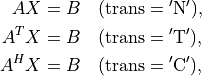
cvxopt.lapack.getrs(A, ipiv, B[, trans = 'N'])

Solves a general set of linear equations

$AX & = B \quad (\mathrm{trans} = \mathrm{'N'}), \\ A^TX & = B \quad (\mathrm{trans} = \mathrm{'T'}), \\ A^HX & = B \quad (\mathrm{trans} = \mathrm{'C'}),$

given the LU factorization computed by gesv or getrf.

On entry, A and ipiv must contain the factorization as computed by gesv or getrf. On entry, B contains the right-hand side $B$ ; on exit it contains the solution $X$ . B must have the same type as A.

cvxopt.lapack.getri(A, ipiv)

Computes the inverse of a matrix.

On entry, A and ipiv must contain the factorization as computed by gesv or getrf. On exit, A contains the matrix inverse.

In the following example we compute

$x = (A^{-1} + A^{-T})b$

for randomly generated problem data, factoring the coefficient matrix once.

>>> from cvxopt import matrix, normal
>>> from cvxopt.lapack import gesv, getrs
>>> n = 10
>>> A = normal(n,n)
>>> b = normal(n)
>>> ipiv = matrix(0, (n,1))
>>> x = +b
>>> gesv(A, x, ipiv)               # x = A^{-1}*b
>>> x2 = +b
>>> getrs(A, ipiv, x2, trans='T')  # x2 = A^{-T}*b
>>> x += x2

Separate functions are provided for equations with band matrices.

cvxopt.lapack.gbsv(A, kl, B[, ipiv = None])

Solves

$A X = B,$

where $A$ and $B$ are real or complex matrices, with $A$ $n$ by $n$ and banded with $k_l$ subdiagonals.

The arguments A and B must have the same type ('d' or 'z'). On entry, B contains the right-hand side $B$ ; on exit it contains the solution $X$ . The optional argument ipiv is an integer matrix of length at least $n$ . If ipiv is provided, then A must have $2k_l + k_u + 1$ rows. On entry the diagonals of $A$ are stored in rows $k_l + 1$ to $2k_l + k_u + 1$ of A, using the BLAS format for general band matrices (see the section Matrix Classes). On exit, the factorization is returned in A and ipiv. If ipiv is not provided, then A must have $k_l + k_u + 1$ rows. On entry the diagonals of $A$ are stored in the rows of A, following the standard BLAS format for general band matrices. In this case, gbsv does not modify A and does not return the factorization.

Raises an ArithmeticError if the matrix is singular.

cvxopt.lapack.gbtrf(A, m, kl, ipiv)

LU factorization of a general $m$ by $n$ real or complex band matrix with $k_l$ subdiagonals.

The matrix is stored using the BLAS format for general band matrices (see the section Matrix Classes), by providing the diagonals (stored as rows of a $k_u + k_l + 1$ by $n$ matrix A), the number of rows $m$ , and the number of subdiagonals $k_l$ . The argument ipiv is an integer matrix of length at least min{ $m$ , $n$ }. On exit, A and ipiv contain the details of the factorization.

Raises an ArithmeticError if the matrix is not full rank.

cvxopt.lapack.gbtrs({A, kl, ipiv, B[, trans = 'N'])

Solves a set of linear equations

$AX & = B \quad (\mathrm{trans} = \mathrm{'N'}), \\ A^TX & = B \quad (\mathrm{trans} = \mathrm{'T'}), \\ A^HX & = B \quad (\mathrm{trans} = \mathrm{'C'}),$

with $A$ a general band matrix with $k_l$ subdiagonals, given the LU factorization computed by gbsv or gbtrf.

On entry, A and ipiv must contain the factorization as computed by gbsv or gbtrf. On entry, B contains the right-hand side $B$ ; on exit it contains the solution $X$ . B must have the same type as A.

As an example, we solve a linear equation with

$A = \left[ \begin{array}{cccc} 1 & 2 & 0 & 0 \\ 3 & 4 & 5 & 0 \\ 6 & 7 & 8 & 9 \\ 0 & 10 & 11 & 12 \end{array}\right], \qquad B = \left[\begin{array}{c} 1 \\ 1 \\ 1 \\ 1 \end{array}\right].$

>>> from cvxopt import matrix
>>> from cvxopt.lapack import gbsv, gbtrf, gbtrs
>>> n, kl, ku = 4, 2, 1
>>> A = matrix([[0., 1., 3., 6.], [2., 4., 7., 10.], [5., 8., 11., 0.], [9., 12., 0., 0.]])
>>> x = matrix(1.0, (n,1))
>>> gbsv(A, kl, x)
>>> print(x)
[ 7.14e-02]
[ 4.64e-01]
[-2.14e-01]
[-1.07e-01]

The code below illustrates how one can reuse the factorization returned by gbsv.

>>> Ac = matrix(0.0, (2*kl+ku+1,n))
>>> Ac[kl:,:] = A
>>> ipiv = matrix(0, (n,1))
>>> x = matrix(1.0, (n,1))
>>> gbsv(Ac, kl, x, ipiv)                 # solves A*x = 1
>>> print(x)
[ 7.14e-02]
[ 4.64e-01]
[-2.14e-01]
[-1.07e-01]
>>> x = matrix(1.0, (n,1))
>>> gbtrs(Ac, kl, ipiv, x, trans='T')     # solve A^T*x = 1
>>> print(x)
[ 7.14e-02]
[ 2.38e-02]
[ 1.43e-01]
[-2.38e-02]

An alternative method uses gbtrf for the factorization.

>>> Ac[kl:,:] = A
>>> gbtrf(Ac, n, kl, ipiv)
>>> x = matrix(1.0, (n,1))
>>> gbtrs(Ac, kl, ipiv, x)                # solve A^T*x = 1
>>> print(x)
[ 7.14e-02]
[ 4.64e-01]
[-2.14e-01]
[-1.07e-01]
>>> x = matrix(1.0, (n,1))
>>> gbtrs(Ac, kl, ipiv, x, trans='T')     # solve A^T*x = 1
>>> print(x)
[ 7.14e-02]
[ 2.38e-02]
[ 1.43e-01]
[-2.38e-02]

The following functions can be used for tridiagonal matrices. They use a simpler matrix format, with the diagonals stored in three separate vectors.

cvxopt.lapack.gtsv(dl, d, du, B))

Solves

$A X = B,$

where $A$ is an $n$ by $n$ tridiagonal matrix.

The subdiagonal of $A$ is stored as a matrix dl of length $n-1$ , the diagonal is stored as a matrix d of length $n$ , and the superdiagonal is stored as a matrix du of length $n-1$ . The four arguments must have the same type ('d' or 'z'). On exit dl, d, du are overwritten with the details of the LU factorization of $A$ . On entry, B contains the right-hand side $B$ ; on exit it contains the solution $X$ .

Raises an ArithmeticError if the matrix is singular.

cvxopt.lapack.gttrf(dl, d, du, du2, ipiv)

LU factorization of an $n$ by $n$ tridiagonal matrix.

The subdiagonal of $A$ is stored as a matrix dl of length $n-1$ , the diagonal is stored as a matrix d of length $n$ , and the superdiagonal is stored as a matrix du of length $n-1$ . dl, d and du must have the same type. du2 is a matrix of length $n-2$ , and of the same type as dl. ipiv is an 'i' matrix of length $n$ . On exit, the five arguments contain the details of the factorization.

Raises an ArithmeticError if the matrix is singular.

cvxopt.lapack.gttrs(dl, d, du, du2, ipiv, B[, trans = 'N'])

Solves a set of linear equations

$AX & = B \quad (\mathrm{trans} = \mathrm{'N'}), \\ A^TX & = B \quad (\mathrm{trans} = \mathrm{'T'}), \\ A^HX & = B \quad (\mathrm{trans} = \mathrm{'C'}),$

where $A$ is an $n$ by $n$ tridiagonal matrix.

The arguments dl, d, du, du2, and ipiv contain the details of the LU factorization as returned by gttrf. On entry, B contains the right-hand side $B$ ; on exit it contains the solution $X$ . B must have the same type as the other arguments.

Positive Definite Linear Equations

cvxopt.lapack.posv(A, B[, uplo = 'L'])

Solves

$A X = B,$

where $A$ is a real symmetric or complex Hermitian positive definite matrix.

On exit, B is replaced by the solution, and A is overwritten with the Cholesky factor. The matrices A and B must have the same type ('d' or 'z').

Raises an ArithmeticError if the matrix is not positive definite.

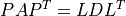
cvxopt.lapack.potrf(A[, uplo = 'L'])

Cholesky factorization

$A = LL^T \qquad \mbox{or} \qquad A = LL^H$

of a positive definite real symmetric or complex Hermitian matrix $A$ .

On exit, the lower triangular part of A (if uplo is 'L') or the upper triangular part (if uplo is 'U') is overwritten with the Cholesky factor or its (conjugate) transpose.

Raises an ArithmeticError if the matrix is not positive definite.

cvxopt.lapack.potrs(A, B[, uplo = 'L'])

Solves a set of linear equations

$AX = B$

with a positive definite real symmetric or complex Hermitian matrix, given the Cholesky factorization computed by posv or potrf.

On entry, A contains the triangular factor, as computed by posv or potrf. On exit, B is replaced by the solution. B must have the same type as A.

cvxopt.lapack.potri(A[, uplo = 'L'])

Computes the inverse of a positive definite matrix.

On entry, A contains the Cholesky factorization computed by potrf or posv. On exit, it contains the matrix inverse.

As an example, we use posv to solve the linear system

(1) $\newcommand{\diag}{\mathop{\bf diag}} \left[ \begin{array}{cc} -\diag(d)^2 & A \\ A^T & 0 \end{array} \right] \left[ \begin{array}{c} x_1 \\ x_2 \end{array} \right] = \left[ \begin{array}{c} b_1 \\ b_2 \end{array} \right]$

by block-elimination. We first pick a random problem.

>>> from cvxopt import matrix, div, normal, uniform
>>> from cvxopt.blas import syrk, gemv
>>> from cvxopt.lapack import posv
>>> m, n = 100, 50
>>> A = normal(m,n)
>>> b1, b2 = normal(m), normal(n)
>>> d = uniform(m)

We then solve the equations

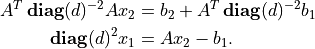
$\newcommand{\diag}{\mathop{\bf diag}} \begin{split} A^T \diag(d)^{-2}A x_2 & = b_2 + A^T \diag(d)^{-2} b_1 \\ \diag(d)^2 x_1 & = Ax_2 - b_1. \end{split}$

>>> Asc = div(A, d[:, n*[0]])                # Asc := diag(d)^{-1}*A
>>> B = matrix(0.0, (n,n))
>>> syrk(Asc, B, trans='T')                  # B := Asc^T * Asc = A^T * diag(d)^{-2} * A
>>> x1 = div(b1, d)                          # x1 := diag(d)^{-1}*b1
>>> x2 = +b2
>>> gemv(Asc, x1, x2, trans='T', beta=1.0)   # x2 := x2 + Asc^T*x1 = b2 + A^T*diag(d)^{-2}*b1
>>> posv(B, x2)                              # x2 := B^{-1}*x2 = B^{-1}*(b2 + A^T*diag(d)^{-2}*b1)
>>> gemv(Asc, x2, x1, beta=-1.0)             # x1 := Asc*x2 - x1 = diag(d)^{-1} * (A*x2 - b1)
>>> x1 = div(x1, d)                          # x1 := diag(d)^{-1}*x1 = diag(d)^{-2} * (A*x2 - b1)

There are separate routines for equations with positive definite band matrices.

cvxopt.lapack.pbsv(A, B[, uplo='L'])

Solves

$AX = B$

where $A$ is a real symmetric or complex Hermitian positive definite band matrix.

On entry, the diagonals of $A$ are stored in A, using the BLAS format for symmetric or Hermitian band matrices (see section Matrix Classes). On exit, B is replaced by the solution, and A is overwritten with the Cholesky factor (in the BLAS format for triangular band matrices). The matrices A and B must have the same type ('d' or 'z').

Raises an ArithmeticError if the matrix is not positive definite.

cvxopt.lapack.pbtrf(A[, uplo = 'L'])

Cholesky factorization

$A = LL^T \qquad \mbox{or} \qquad A = LL^H$

of a positive definite real symmetric or complex Hermitian band matrix $A$ .

On entry, the diagonals of $A$ are stored in A, using the BLAS format for symmetric or Hermitian band matrices. On exit, A contains the Cholesky factor, in the BLAS format for triangular band matrices.

Raises an ArithmeticError if the matrix is not positive definite.

cvxopt.lapack.pbtrs(A, B[, uplo = 'L'])

Solves a set of linear equations

$AX=B$

with a positive definite real symmetric or complex Hermitian band matrix, given the Cholesky factorization computed by pbsv or pbtrf.

On entry, A contains the triangular factor, as computed by pbsv or pbtrf. On exit, B is replaced by the solution. B must have the same type as A.

The following functions are useful for tridiagonal systems.

cvxopt.lapack.ptsv(d, e, B)

Solves

$A X = B,$

where $A$ is an $n$ by $n$ positive definite real symmetric or complex Hermitian tridiagonal matrix.

The diagonal of $A$ is stored as a 'd' matrix d of length $n$ and its subdiagonal as a 'd' or 'z' matrix e of length $n-1$ . The arguments e and B must have the same type. On exit d contains the diagonal elements of $D$ in the LDL^T or LDL^H factorization of $A$ , and e contains the subdiagonal elements of the unit lower bidiagonal matrix $L$ . B is overwritten with the solution $X$ . Raises an ArithmeticError if the matrix is singular.

cvxopt.lapack.pttrf(d, e)

LDL^T or LDL^H factorization of an $n$ by $n$ positive definite real symmetric or complex Hermitian tridiagonal matrix $A$ .

On entry, the argument d is a 'd' matrix with the diagonal elements of $A$ . The argument e is 'd' or 'z' matrix containing the subdiagonal of $A$ . On exit d contains the diagonal elements of $D$ , and e contains the subdiagonal elements of the unit lower bidiagonal matrix $L$ .

Raises an ArithmeticError if the matrix is singular.

cvxopt.lapack.pttrs(d, e, B[, uplo = 'L'])

Solves a set of linear equations

$AX = B$

where $A$ is an $n$ by $n$ positive definite real symmetric or complex Hermitian tridiagonal matrix, given its LDL^T or LDL^H factorization.

The argument d is the diagonal of the diagonal matrix $D$ . The argument uplo only matters for complex matrices. If uplo is 'L', then on exit e contains the subdiagonal elements of the unit bidiagonal matrix $L$ . If uplo is 'U', then e contains the complex conjugates of the elements of the unit bidiagonal matrix $L$ . On exit, B is overwritten with the solution $X$ . B must have the same type as e.

Symmetric and Hermitian Linear Equations

cvxopt.lapack.sysv(A, B[, ipiv = None, uplo = 'L'])

Solves

$AX = B$

where $A$ is a real or complex symmetric matrix of order $n$ .

On exit, B is replaced by the solution. The matrices A and B must have the same type ('d' or 'z'). The optional argument ipiv is an integer matrix of length at least equal to $n$ . If ipiv is provided, sysv solves the system and returns the factorization in A and ipiv. If ipiv is not specified, sysv solves the system but does not return the factorization and does not modify A.

Raises an ArithmeticError if the matrix is singular.

cvxopt.lapack.sytrf(A, ipiv[, uplo = 'L'])

LDL^T factorization

$PAP^T = LDL^T$

of a real or complex symmetric matrix $A$ of order $n$ .

ipiv is an 'i' matrix of length at least $n$ . On exit, A and ipiv contain the factorization.

Raises an ArithmeticError if the matrix is singular.

cvxopt.lapack.sytrs(A, ipiv, B[, uplo = 'L'])

Solves

$A X = B$

given the LDL^T factorization computed by sytrf or sysv. B must have the same type as A.

cvxopt.lapack.sytri(A, ipiv[, uplo = 'L'])

Computes the inverse of a real or complex symmetric matrix.

On entry, A and ipiv contain the LDL^T factorization computed by sytrf or sysv. On exit, A contains the inverse.

cvxopt.lapack.hesv(A, B[, ipiv = None, uplo = 'L'])

Solves

$A X = B$

where $A$ is a real symmetric or complex Hermitian of order $n$ .

On exit, B is replaced by the solution. The matrices A and B must have the same type ('d' or 'z'). The optional argument ipiv is an integer matrix of length at least $n$ . If ipiv is provided, then hesv solves the system and returns the factorization in A and ipiv. If ipiv is not specified, then hesv solves the system but does not return the factorization and does not modify A.

Raises an ArithmeticError if the matrix is singular.

cvxopt.lapack.hetrf(A, ipiv[, uplo = 'L'])

LDL^H factorization

$PAP^T = LDL^H$

of a real symmetric or complex Hermitian matrix of order $n$ . ipiv is an 'i' matrix of length at least $n$ . On exit, A and ipiv contain the factorization.

Raises an ArithmeticError if the matrix is singular.

cvxopt.lapack.hetrs(A, ipiv, B[, uplo = 'L'])

Solves

$A X = B$

given the LDL^H factorization computed by hetrf or hesv.

cvxopt.lapack.hetri(A, ipiv[, uplo = 'L'])

Computes the inverse of a real symmetric or complex Hermitian matrix.

On entry, A and ipiv contain the LDL^H factorization computed by hetrf or hesv. On exit, A contains the inverse.

As an example we solve the KKT system (1).

>>> from cvxopt.lapack import sysv
>>> K = matrix(0.0, (m+n,m+n))
>>> K[: (m+n)*m : m+n+1] = -d**2
>>> K[:m, m:] = A
>>> x = matrix(0.0, (m+n,1))
>>> x[:m], x[m:] = b1, b2
>>> sysv(K, x, uplo='U')

Triangular Linear Equations

cvxopt.lapack.trtrs(A, B[, uplo = 'L', trans = 'N', diag = 'N'])

Solves a triangular set of equations

$AX & = B \quad (\mathrm{trans} = \mathrm{'N'}), \\ A^TX & = B \quad (\mathrm{trans} = \mathrm{'T'}), \\ A^HX & = B \quad (\mathrm{trans} = \mathrm{'C'}),$

where $A$ is real or complex and triangular of order $n$ , and $B$ is a matrix with $n$ rows.

A and B are matrices with the same type ('d' or 'z'). trtrs is similar to blas.trsm, except that it raises an ArithmeticError if a diagonal element of A is zero (whereas blas.trsm returns inf values).

cvxopt.lapack.trtri(A[, uplo = 'L', diag = 'N']): Computes the inverse of a real or complex triangular matrix $A$ . On exit, A contains the inverse.

cvxopt.lapack.tbtrs(A, B[, uplo = 'L', trans = 'T', diag = 'N'])

Solves a triangular set of equations

$AX & = B \quad (\mathrm{trans} = \mathrm{'N'}), \\ A^TX & = B \quad (\mathrm{trans} = \mathrm{'T'}), \\ A^HX & = B \quad (\mathrm{trans} = \mathrm{'C'}),$

where $A$ is real or complex triangular band matrix of order $n$ , and $B$ is a matrix with $n$ rows.

The diagonals of $A$ are stored in A using the BLAS conventions for triangular band matrices. A and B are matrices with the same type ('d' or 'z'). On exit, B is replaced by the solution $X$ .

Least-Squares and Least-Norm Problems

cvxopt.lapack.gels(A, B[, trans = 'N'])

Solves least-squares and least-norm problems with a full rank $m$ by $n$ matrix $A$ .

trans is 'N'. If $m$ is greater than or equal to $n$ , gels solves the least-squares problem

$\begin{array}{ll} \mbox{minimize} & \|AX-B\|_F. \end{array}$

If $m$ is less than or equal to $n$ , gels solves the least-norm problem

$\begin{array}{ll} \mbox{minimize} & \|X\|_F \\ \mbox{subject to} & AX = B. \end{array}$
trans is 'T' or 'C' and A and B are real. If $m$ is greater than or equal to $n$ , gels solves the least-norm problem

$\begin{array}{ll} \mbox{minimize} & \|X\|_F \\ \mbox{subject to} & A^TX=B. \end{array}$

If $m$ is less than or equal to $n$ , gels solves the least-squares problem

$\begin{array}{ll} \mbox{minimize} & \|A^TX-B\|_F. \end{array}$
trans is 'C' and A and B are complex. If $m$ is greater than or equal to $n$ , gels solves the least-norm problem

$\begin{array}{ll} \mbox{minimize} & \|X\|_F \\ \mbox{subject to} & A^HX=B. \end{array}$

If $m$ is less than or equal to $n$ , gels solves the least-squares problem

$\begin{array}{ll} \mbox{minimize} & \|A^HX-B\|_F. \end{array}$

A and B must have the same typecode ('d' or 'z'). trans = 'T' is not allowed if A is complex. On exit, the solution $X$ is stored as the leading submatrix of B. The matrix A is overwritten with details of the QR or the LQ factorization of $A$ .

Note that gels does not check whether $A$ is full rank.

The following functions compute QR and LQ factorizations.

cvxopt.lapack.geqrf(A, tau)

QR factorization of a real or complex matrix A:

$A = Q R.$

If $A$ is $m$ by $n$ , then $Q$ is $m$ by $m$ and orthogonal/unitary, and $R$ is $m$ by $n$ and upper triangular (if $m$ is greater than or equal to $n$ ), or upper trapezoidal (if $m$ is less than or equal to $n$ ).

tau is a matrix of the same type as A and of length min{ $m$ , $n$ }. On exit, $R$ is stored in the upper triangular/trapezoidal part of A. The matrix $Q$ is stored as a product of min{ $m$ , $n$ } elementary reflectors in the first min{ $m$ , $n$ } columns of A and in tau.

cvxopt.lapack.gelqf(A, tau)

LQ factorization of a real or complex matrix A:

$A = L Q.$

If $A$ is $m$ by $n$ , then $Q$ is $n$ by $n$ and orthogonal/unitary, and $L$ is $m$ by $n$ and lower triangular (if $m$ is less than or equal to $n$ ), or lower trapezoidal (if $m$ is greater than or equal to $n$ ).

tau is a matrix of the same type as A and of length min{ $m$ , $n$ }. On exit, $L$ is stored in the lower triangular/trapezoidal part of A. The matrix $Q$ is stored as a product of min{ $m$ , $n$ } elementary reflectors in the first min{ $m$ , $n$ } rows of A and in tau.

cvxopt.lapack.geqp3(A, jpvt, tau)

QR factorization with column pivoting of a real or complex matrix $A$ :

$A P = Q R.$

If $A$ is $m$ by $n$ , then $Q$ is $m$ by $m$ and orthogonal/unitary, and $R$ is $m$ by $n$ and upper triangular (if $m$ is greater than or equal to $n$ ), or upper trapezoidal (if $m$ is less than or equal to $n$ ).

tau is a matrix of the same type as A and of length min{ $m$ , $n$ }. jpvt is an integer matrix of length $n$ . On entry, if jpvt[k] is nonzero, then column $k$ of $A$ is permuted to the front of $AP$ . Otherwise, column $k$ is a free column.

On exit, jpvt contains the permutation $P$ : the operation $AP$ is equivalent to A[:, jpvt-1]. $R$ is stored in the upper triangular/trapezoidal part of A. The matrix $Q$ is stored as a product of min{ $m$ , $n$ } elementary reflectors in the first min{ $m$ ,:math:n} columns of A and in tau.

In most applications, the matrix $Q$ is not needed explicitly, and it is sufficient to be able to make products with $Q$ or its transpose. The functions unmqr and ormqr multiply a matrix with the orthogonal matrix computed by geqrf.

cvxopt.lapack.unmqr(A, tau, C[, side = 'L', trans = 'N'])

Product with a real orthogonal or complex unitary matrix:

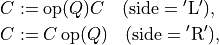
$\newcommand{\op}{\mathop{\mathrm{op}}} \begin{split} C & := \op(Q)C \quad (\mathrm{side} = \mathrm{'L'}), \\ C & := C\op(Q) \quad (\mathrm{side} = \mathrm{'R'}), \\ \end{split}$

where

$\newcommand{\op}{\mathop{\mathrm{op}}} \op(Q) = \left\{ \begin{array}{ll} Q & \mathrm{trans} = \mathrm{'N'} \\ Q^T & \mathrm{trans} = \mathrm{'T'} \\ Q^H & \mathrm{trans} = \mathrm{'C'}. \end{array}\right.$

If A is $m$ by $n$ , then $Q$ is square of order $m$ and orthogonal or unitary. $Q$ is stored in the first min{ $m$ , $n$ } columns of A and in tau as a product of min{ $m$ , $n$ } elementary reflectors, as computed by geqrf. The matrices A, tau, and C must have the same type. trans = 'T' is only allowed if the typecode is 'd'.

cvxopt.lapack.ormqr(A, tau, C[, side = 'L', trans = 'N']): Identical to unmqr but works only for real matrices, and the possible values of trans are 'N' and 'T'.

As an example, we solve a least-squares problem by a direct call to gels, and by separate calls to geqrf, ormqr, and trtrs.

>>> from cvxopt import blas, lapack, matrix, normal
>>> m, n = 10, 5
>>> A, b = normal(m,n), normal(m,1)
>>> x1 = +b
>>> lapack.gels(+A, x1)                  # x1[:n] minimizes || A*x - b ||_2
>>> tau = matrix(0.0, (n,1))
>>> lapack.geqrf(A, tau)                 # A = [Q1, Q2] * [R1; 0]
>>> x2 = +b
>>> lapack.ormqr(A, tau, x2, trans='T')  # x2 := [Q1, Q2]' * x2
>>> lapack.trtrs(A[:n,:], x2, uplo='U')  # x2[:n] := R1^{-1} * x2[:n]
>>> blas.nrm2(x1[:n] - x2[:n])
3.0050798580569307e-16

The next two functions make products with the orthogonal matrix computed by gelqf.

cvxopt.lapack.unmlq(A, tau, C[, side = 'L', trans = 'N'])

Product with a real orthogonal or complex unitary matrix:

$\newcommand{\op}{\mathop{\mathrm{op}}} \begin{split} C & := \op(Q)C \quad (\mathrm{side} = \mathrm{'L'}), \\ C & := C\op(Q) \quad (\mathrm{side} = \mathrm{'R'}), \\ \end{split}$

where

$\newcommand{\op}{\mathop{\mathrm{op}}} \op(Q) = \left\{ \begin{array}{ll} Q & \mathrm{trans} = \mathrm{'N'}, \\ Q^T & \mathrm{trans} = \mathrm{'T'}, \\ Q^H & \mathrm{trans} = \mathrm{'C'}. \end{array}\right.$

If A is $m$ by $n$ , then $Q$ is square of order $n$ and orthogonal or unitary. $Q$ is stored in the first min{ $m$ , $n$ } rows of A and in tau as a product of min{ $m$ , $n$ } elementary reflectors, as computed by gelqf. The matrices A, tau, and C must have the same type. trans = 'T' is only allowed if the typecode is 'd'.

cvxopt.lapack.ormlq(A, tau, C[, side = 'L', trans = 'N']): Identical to unmlq but works only for real matrices, and the possible values of trans or 'N' and 'T'.

As an example, we solve a least-norm problem by a direct call to gels, and by separate calls to gelqf, ormlq, and trtrs.

>>> from cvxopt import blas, lapack, matrix, normal
>>> m, n = 5, 10
>>> A, b = normal(m,n), normal(m,1)
>>> x1 = matrix(0.0, (n,1))
>>> x1[:m] = b
>>> lapack.gels(+A, x1)                  # x1 minimizes ||x||_2 subject to A*x = b
>>> tau = matrix(0.0, (m,1))
>>> lapack.gelqf(A, tau)                 # A = [L1, 0] * [Q1; Q2]
>>> x2 = matrix(0.0, (n,1))
>>> x2[:m] = b                           # x2 = [b; 0]
>>> lapack.trtrs(A[:,:m], x2)            # x2[:m] := L1^{-1} * x2[:m]
>>> lapack.ormlq(A, tau, x2, trans='T')  # x2 := [Q1, Q2]' * x2
>>> blas.nrm2(x1 - x2)
0.0

Finally, if the matrix $Q$ is needed explicitly, it can be generated from the output of geqrf and gelqf using one of the following functions.

cvxopt.lapack.ungqr(A, tau): If A has size $m$ by $n$ , and tau has length $k$ , then, on entry, the first k columns of the matrix A and the entries of tau contai an unitary or orthogonal matrix $Q$ of order $m$ , as computed by geqrf. On exit, the first min{ $m$ , $n$ } columns of $Q$ are contained in the leading columns of A.

cvxopt.lapack.orgqr(A, tau): Identical to ungqr but works only for real matrices.

cvxopt.lapack.unglq(A, tau): If A has size $m$ by $n$ , and tau has length $k$ , then, on entry, the first k rows of the matrix A and the entries of tau contain a unitary or orthogonal matrix $Q$ of order $n$ , as computed by gelqf. On exit, the first min{ $m$ , $n$ } rows of $Q$ are contained in the leading rows of A.

cvxopt.lapack.orglq(A, tau): Identical to unglq but works only for real matrices.

We illustrate this with the QR factorization of the matrix

$A = \left[\begin{array}{rrr} 6 & -5 & 4 \\ 6 & 3 & -4 \\ 19 & -2 & 7 \\ 6 & -10 & -5 \end{array} \right] = \left[\begin{array}{cc} Q_1 & Q_2 \end{array}\right] \left[\begin{array}{c} R \\ 0 \end{array}\right].$

>>> from cvxopt import matrix, lapack
>>> A = matrix([ [6., 6., 19., 6.], [-5., 3., -2., -10.], [4., -4., 7., -5] ])
>>> m, n = A.size
>>> tau = matrix(0.0, (n,1))
>>> lapack.geqrf(A, tau)
>>> print(A[:n, :])              # Upper triangular part is R.
[-2.17e+01  5.08e+00 -4.76e+00]
[ 2.17e-01 -1.06e+01 -2.66e+00]
[ 6.87e-01  3.12e-01 -8.74e+00]
>>> Q1 = +A
>>> lapack.orgqr(Q1, tau)
>>> print(Q1)
[-2.77e-01  3.39e-01 -4.10e-01]
[-2.77e-01 -4.16e-01  7.35e-01]
[-8.77e-01 -2.32e-01 -2.53e-01]
[-2.77e-01  8.11e-01  4.76e-01]
>>> Q = matrix(0.0, (m,m))
>>> Q[:, :n] = A
>>> lapack.orgqr(Q, tau)
>>> print(Q)                     # Q = [ Q1, Q2]
[-2.77e-01  3.39e-01 -4.10e-01 -8.00e-01]
[-2.77e-01 -4.16e-01  7.35e-01 -4.58e-01]
[-8.77e-01 -2.32e-01 -2.53e-01  3.35e-01]
[-2.77e-01  8.11e-01  4.76e-01  1.96e-01]

The orthogonal matrix in the factorization

$A = \left[ \begin{array}{rrrr} 3 & -16 & -10 & -1 \\ -2 & -12 & -3 & 4 \\ 9 & 19 & 6 & -6 \end{array}\right] = Q \left[\begin{array}{cc} R_1 & R_2 \end{array}\right]$

can be generated as follows.

>>> A = matrix([ [3., -2., 9.], [-16., -12., 19.], [-10., -3., 6.], [-1., 4., -6.] ])
>>> m, n = A.size
>>> tau = matrix(0.0, (m,1))
>>> lapack.geqrf(A, tau)
>>> R = +A
>>> print(R)                     # Upper trapezoidal part is [R1, R2].
[-9.70e+00 -1.52e+01 -3.09e+00  6.70e+00]
[-1.58e-01  2.30e+01  1.14e+01 -1.92e+00]
[ 7.09e-01 -5.57e-01  2.26e+00  2.09e+00]
>>> lapack.orgqr(A, tau)
>>> print(A[:, :m])              # Q is in the first m columns of A.
[-3.09e-01 -8.98e-01 -3.13e-01]
[ 2.06e-01 -3.85e-01  9.00e-01]
[-9.28e-01  2.14e-01  3.04e-01]

Symmetric and Hermitian Eigenvalue Decomposition

The first four routines compute all or selected eigenvalues and eigenvectors of a real symmetric matrix $A$ :

$\newcommand{\diag}{\mathop{\bf diag}} A = V\diag(\lambda)V^T,\qquad V^TV = I.$

cvxopt.lapack.syev(A, W[, jobz = 'N', uplo = 'L'])

Eigenvalue decomposition of a real symmetric matrix of order $n$ .

W is a real matrix of length at least $n$ . On exit, W contains the eigenvalues in ascending order. If jobz is 'V', the eigenvectors are also computed and returned in A. If jobz is 'N', the eigenvectors are not returned and the contents of A are destroyed.

Raises an ArithmeticError if the eigenvalue decomposition fails.

cvxopt.lapack.syevd(A, W[, jobz = 'N', uplo = 'L']): This is an alternative to syev, based on a different algorithm. It is faster on large problems, but also uses more memory.

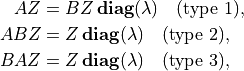
cvxopt.lapack.syevx(A, W[, jobz = 'N', range = 'A', uplo = 'L', vl = 0.0, vu = 0.0, il = 1, iu = 1, Z = None])

Computes selected eigenvalues and eigenvectors of a real symmetric matrix of order $n$ .

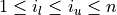W is a real matrix of length at least $n$ . On exit, W contains the eigenvalues in ascending order. If range is 'A', all the eigenvalues are computed. If range is 'I', eigenvalues $i_l$ through $i_u$ are computed, where $1 \leq i_l \leq i_u \leq n$ . If range is 'V', the eigenvalues in the interval $(v_l, v_u]$ are computed.

If jobz is 'V', the (normalized) eigenvectors are computed, and returned in Z. If jobz is 'N', the eigenvectors are not computed. In both cases, the contents of A are destroyed on exit.

Z is optional (and not referenced) if jobz is 'N'. It is required if jobz is 'V' and must have at least $n$ columns if range is 'A' or 'V' and at least $i_u - i_l + 1$ columns if range is 'I'.

syevx returns the number of computed eigenvalues.

cvxopt.lapack.syevr(A, W[, jobz = 'N', range = 'A', uplo = 'L', vl = 0.0, vu = 0.0, il = 1, iu = n, Z = None]): This is an alternative to syevx. syevr is the most recent LAPACK routine for symmetric eigenvalue problems, and expected to supersede the three other routines in future releases.

The next four routines can be used to compute eigenvalues and eigenvectors for complex Hermitian matrices:

$\newcommand{\diag}{\mathop{\bf diag}} A = V\diag(\lambda)V^H,\qquad V^HV = I.$

For real symmetric matrices they are identical to the corresponding syev* routines.

cvxopt.lapack.heev(A, W[, jobz = 'N', uplo = 'L'])

Eigenvalue decomposition of a real symmetric or complex Hermitian matrix of order $n$ .

The calling sequence is identical to syev, except that A can be real or complex.

cvxopt.lapack.heevd(A, W[, jobz = 'N'[, uplo = 'L']]): This is an alternative to heev.

cvxopt.lapack.heevx(A, W[, jobz = 'N', range = 'A', uplo = 'L', vl = 0.0, vu = 0.0, il = 1, iu = n, Z = None])

Computes selected eigenvalues and eigenvectors of a real symmetric or complex Hermitian matrix.

The calling sequence is identical to syevx, except that A can be real or complex. Z must have the same type as A.

cvxopt.lapack.heevr(A, W[, jobz = 'N', range = 'A', uplo = 'L', vl = 0.0, vu = 0.0, il = 1, iu = n, Z = None]): This is an alternative to heevx.

Generalized Symmetric Definite Eigenproblems

Three types of generalized eigenvalue problems can be solved:

(2) $\newcommand{\diag}{\mathop{\bf diag}} \begin{split} AZ & = BZ\diag(\lambda)\quad \mbox{(type 1)}, \\ ABZ & = Z\diag(\lambda) \quad \mbox{(type 2)}, \\ BAZ & = Z\diag(\lambda) \quad \mbox{(type 3)}, \end{split}$

with $A$ and $B$ real symmetric or complex Hermitian, and $B$ is positive definite. The matrix of eigenvectors is normalized as follows:

$Z^H BZ = I \quad \mbox{(types 1 and 2)}, \qquad Z^H B^{-1}Z = I \quad \mbox{(type 3)}.$

cvxopt.lapack.sygv(A, B, W[, itype = 1, jobz = 'N', uplo = 'L']): Solves the generalized eigenproblem (2) for real symmetric matrices of order $n$ , stored in real matrices A and B. itype is an integer with possible values 1, 2, 3, and specifies the type of eigenproblem. W is a real matrix of length at least $n$ . On exit, it contains the eigenvalues in ascending order. On exit, B contains the Cholesky factor of $B$ . If jobz is 'V', the eigenvectors are computed and returned in A. If jobz is 'N', the eigenvectors are not returned and the contents of A are destroyed.

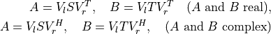
cvxopt.lapack.hegv(A, B, W[, itype = 1, jobz = 'N', uplo = 'L']): Generalized eigenvalue problem (2) of real symmetric or complex Hermitian matrix of order $n$ . The calling sequence is identical to sygv, except that A and B can be real or complex.

Singular Value Decomposition

cvxopt.lapack.gesvd(A, S[, jobu = 'N', jobvt = 'N', U = None, Vt = None])

Singular value decomposition

$A = U \Sigma V^T, \qquad A = U \Sigma V^H$

of a real or complex $m$ by $n$ matrix $A$ .

S is a real matrix of length at least min{ $m$ , $n$ }. On exit, its first min{ $m$ , $n$ } elements are the singular values in descending order.

The argument jobu controls how many left singular vectors are computed. The possible values are 'N', 'A', 'S' and 'O'. If jobu is 'N', no left singular vectors are computed. If jobu is 'A', all left singular vectors are computed and returned as columns of U. If jobu is 'S', the first min{ $m$ , $n$ } left singular vectors are computed and returned as columns of U. If jobu is 'O', the first min{ $m$ , $n$ } left singular vectors are computed and returned as columns of A. The argument U is None(if jobu is 'N' or 'A') or a matrix of the same type as A.

The argument jobvt controls how many right singular vectors are computed. The possible values are 'N', 'A', 'S' and 'O'. If jobvt is 'N', no right singular vectors are computed. If jobvt is 'A', all right singular vectors are computed and returned as rows of Vt. If jobvt is 'S', the first min{ $m$ , $n$ } right singular vectors are computed and their (conjugate) transposes are returned as rows of Vt. If jobvt is 'O', the first min{ $m$ , $n$ } right singular vectors are computed and their (conjugate) transposes are returned as rows of A. Note that the (conjugate) transposes of the right singular vectors (i.e., the matrix $V^H$ ) are returned in Vt or A. The argument Vt can be None (if jobvt is 'N' or 'A') or a matrix of the same type as A.

On exit, the contents of A are destroyed.

cvxopt.lapack.gesdd(A, S[, jobz = 'N', U = None, Vt = None])

Singular value decomposition of a real or complex $m$ by $n$ matrix.. This function is based on a divide-and-conquer algorithm and is faster than gesvd.

S is a real matrix of length at least min{ $m$ , $n$ }. On exit, its first min{ $m$ , $n$ } elements are the singular values in descending order.

The argument jobz controls how many singular vectors are computed. The possible values are 'N', 'A', 'S' and 'O'. If jobz is 'N', no singular vectors are computed. If jobz is 'A', all $m$ left singular vectors are computed and returned as columns of U and all $n$ right singular vectors are computed and returned as rows of Vt. If jobz is 'S', the first min{ $m$ , $n$ } left and right singular vectors are computed and returned as columns of U and rows of Vt. If jobz is 'O' and $m$ is greater than or equal to $n$ , the first $n$ left singular vectors are returned as columns of A and the $n$ right singular vectors are returned as rows of Vt. If jobz is 'O' and $m$ is less than $n$ , the $m$ left singular vectors are returned as columns of U and the first $m$ right singular vectors are returned as rows of A. Note that the (conjugate) transposes of the right singular vectors are returned in Vt or A.

The argument U can be None (if jobz is 'N' or 'A' of jobz is 'O' and $m$ is greater than or equal to $n$ ) or a matrix of the same type as A. The argument Vt can be None(if jobz is 'N' or 'A' or jobz is 'O' and :math`m` is less than $n$ ) or a matrix of the same type as A.

On exit, the contents of A are destroyed.

Schur and Generalized Schur Factorization

cvxopt.lapack.gees(A[, w = None, V = None, select = None])

Computes the Schur factorization

$A = V S V^T \quad \mbox{($A$ real)}, \qquad A = V S V^H \quad \mbox{($A$ complex)}$

of a real or complex $n$ by $n$ matrix $A$ .

If $A$ is real, the matrix of Schur vectors $V$ is orthogonal, and $S$ is a real upper quasi-triangular matrix with 1 by 1 or 2 by 2 diagonal blocks. The 2 by 2 blocks correspond to complex conjugate pairs of eigenvalues of $A$ . If $A$ is complex, the matrix of Schur vectors $V$ is unitary, and $S$ is a complex upper triangular matrix with the eigenvalues of $A$ on the diagonal.

The optional argument w is a complex matrix of length at least $n$ . If it is provided, the eigenvalues of A are returned in w. The optional argument V is an $n$ by $n$ matrix of the same type as A. If it is provided, then the Schur vectors are returned in V.

The argument select is an optional ordering routine. It must be a Python function that can be called as f(s) with a complex argument s, and returns True or False. The eigenvalues for which select returns True will be selected to appear first along the diagonal. (In the real Schur factorization, if either one of a complex conjugate pair of eigenvalues is selected, then both are selected.)

On exit, A is replaced with the matrix $S$ . The function gees returns an integer equal to the number of eigenvalues that were selected by the ordering routine. If select is None, then gees returns 0.

As an example we compute the complex Schur form of the matrix

$A = \left[\begin{array}{rrrrr} -7 & -11 & -6 & -4 & 11 \\ 5 & -3 & 3 & -12 & 0 \\ 11 & 11 & -5 & -14 & 9 \\ -4 & 8 & 0 & 8 & 6 \\ 13 & -19 & -12 & -8 & 10 \end{array}\right].$

>>> A = matrix([[-7., 5., 11., -4., 13.], [-11., -3., 11., 8., -19.], [-6., 3., -5., 0., -12.],
                [-4., -12., -14., 8., -8.], [11., 0., 9., 6., 10.]])
>>> S = matrix(A, tc='z')
>>> w = matrix(0.0, (5,1), 'z')
>>> lapack.gees(S, w)
0
>>> print(S)
[ 5.67e+00+j1.69e+01 -2.13e+01+j2.85e+00  1.40e+00+j5.88e+00 -4.19e+00+j2.05e-01  3.19e+00-j1.01e+01]
[ 0.00e+00-j0.00e+00  5.67e+00-j1.69e+01  1.09e+01+j5.93e-01 -3.29e+00-j1.26e+00 -1.26e+01+j7.80e+00]
[ 0.00e+00-j0.00e+00  0.00e+00-j0.00e+00  1.27e+01+j3.43e-17 -6.83e+00+j2.18e+00  5.31e+00-j1.69e+00]
[ 0.00e+00-j0.00e+00  0.00e+00-j0.00e+00  0.00e+00-j0.00e+00 -1.31e+01-j0.00e+00 -2.60e-01-j0.00e+00]
[ 0.00e+00-j0.00e+00  0.00e+00-j0.00e+00  0.00e+00-j0.00e+00  0.00e+00-j0.00e+00 -7.86e+00-j0.00e+00]
>>> print(w)
[ 5.67e+00+j1.69e+01]
[ 5.67e+00-j1.69e+01]
[ 1.27e+01+j3.43e-17]
[-1.31e+01-j0.00e+00]
[-7.86e+00-j0.00e+00]

An ordered Schur factorization with the eigenvalues in the left half of the complex plane ordered first, can be computed as follows.

>>> S = matrix(A, tc='z')
>>> def F(x): return (x.real < 0.0)
...
>>> lapack.gees(S, w, select = F)
2
>>> print(S)
[-1.31e+01-j0.00e+00 -1.72e-01+j7.93e-02 -2.81e+00+j1.46e+00  3.79e+00-j2.67e-01  5.14e+00-j4.84e+00]
[ 0.00e+00-j0.00e+00 -7.86e+00-j0.00e+00 -1.43e+01+j8.31e+00  5.17e+00+j8.79e+00  2.35e+00-j7.86e-01]
[ 0.00e+00-j0.00e+00  0.00e+00-j0.00e+00  5.67e+00+j1.69e+01 -1.71e+01-j1.41e+01  1.83e+00-j4.63e+00]
[ 0.00e+00-j0.00e+00  0.00e+00-j0.00e+00  0.00e+00-j0.00e+00  5.67e+00-j1.69e+01 -8.75e+00+j2.88e+00]
[ 0.00e+00-j0.00e+00  0.00e+00-j0.00e+00  0.00e+00-j0.00e+00  0.00e+00-j0.00e+00  1.27e+01+j3.43e-17]
>>> print(w)
[-1.31e+01-j0.00e+00]
[-7.86e+00-j0.00e+00]
[ 5.67e+00+j1.69e+01]
[ 5.67e+00-j1.69e+01]
[ 1.27e+01+j3.43e-17]

cvxopt.lapack.gges(A, B[, a = None, b = None, Vl = None, Vr = None, select = None])

Computes the generalized Schur factorization

$A = V_l S V_r^T, \quad B = V_l T V_r^T \quad \mbox{($A$ and $B$ real)}, A = V_l S V_r^H, \quad B = V_l T V_r^H, \quad \mbox{($A$ and $B$ complex)}$

of a pair of real or complex $n$ by $n$ matrices $A$ , $B$ .

If $A$ and $B$ are real, then the matrices of left and right Schur vectors $V_l$ and $V_r$ are orthogonal, $S$ is a real upper quasi-triangular matrix with 1 by 1 or 2 by 2 diagonal blocks, and $T$ is a real triangular matrix with nonnegative diagonal. The 2 by 2 blocks along the diagonal of $S$ correspond to complex conjugate pairs of generalized eigenvalues of $A$ , $B$ . If $A$ and $B$ are complex, the matrices of left and right Schur vectors $V_l$ and $V_r$ are unitary, $S$ is complex upper triangular, and $T$ is complex upper triangular with nonnegative real diagonal.

The optional arguments a and b are 'z' and 'd' matrices of length at least $n$ . If these are provided, the generalized eigenvalues of A, B are returned in a and b. (The generalized eigenvalues are the ratios a[k] / b[k].) The optional arguments Vl and Vr are $n$ by $n$ matrices of the same type as A and B. If they are provided, then the left Schur vectors are returned in Vl and the right Schur vectors are returned in Vr.

The argument select is an optional ordering routine. It must be a Python function that can be called as f(x,y) with a complex argument x and a real argument y, and returns True or False. The eigenvalues for which select returns True will be selected to appear first on the diagonal. (In the real Schur factorization, if either one of a complex conjugate pair of eigenvalues is selected, then both are selected.)

On exit, A is replaced with the matrix $S$ and B is replaced with the matrix $T$ . The function gges returns an integer equal to the number of eigenvalues that were selected by the ordering routine. If select is None, then gges returns 0.

As an example, we compute the generalized complex Schur form of the matrix $A$ of the previous example, and

$B = \left[\begin{array}{ccccc} 1 & 0 & 0 & 0 & 0 \\ 0 & 1 & 0 & 0 & 0 \\ 0 & 0 & 1 & 0 & 0 \\ 0 & 0 & 0 & 1 & 0 \\ 0 & 0 & 0 & 0 & 0 \end{array}\right].$

>>> A = matrix([[-7., 5., 11., -4., 13.], [-11., -3., 11., 8., -19.], [-6., 3., -5., 0., -12.],
                [-4., -12., -14., 8., -8.], [11., 0., 9., 6., 10.]])
>>> B = matrix(0.0, (5,5))
>>> B[:19:6] = 1.0
>>> S = matrix(A, tc='z')
>>> T = matrix(B, tc='z')
>>> a = matrix(0.0, (5,1), 'z')
>>> b = matrix(0.0, (5,1))
>>> lapack.gges(S, T, a, b)
0
>>> print(S)
[ 6.64e+00-j8.87e+00 -7.81e+00-j7.53e+00  6.16e+00-j8.51e-01  1.18e+00+j9.17e+00  5.88e+00-j4.51e+00]
[ 0.00e+00-j0.00e+00  8.48e+00+j1.13e+01 -2.12e-01+j1.00e+01  5.68e+00+j2.40e+00 -2.47e+00+j9.38e+00]
[ 0.00e+00-j0.00e+00  0.00e+00-j0.00e+00 -1.39e+01-j0.00e+00  6.78e+00-j0.00e+00  1.09e+01-j0.00e+00]
[ 0.00e+00-j0.00e+00  0.00e+00-j0.00e+00  0.00e+00-j0.00e+00 -6.62e+00-j0.00e+00 -2.28e-01-j0.00e+00]
[ 0.00e+00-j0.00e+00  0.00e+00-j0.00e+00  0.00e+00-j0.00e+00  0.00e+00-j0.00e+00 -2.89e+01-j0.00e+00]
>>> print(T)
[ 6.46e-01-j0.00e+00  4.29e-01-j4.79e-02  2.02e-01-j3.71e-01  1.08e-01-j1.98e-01 -1.95e-01+j3.58e-01]
[ 0.00e+00-j0.00e+00  8.25e-01-j0.00e+00 -2.17e-01+j3.11e-01 -1.16e-01+j1.67e-01  2.10e-01-j3.01e-01]
[ 0.00e+00-j0.00e+00  0.00e+00-j0.00e+00  7.41e-01-j0.00e+00 -3.25e-01-j0.00e+00  5.87e-01-j0.00e+00]
[ 0.00e+00-j0.00e+00  0.00e+00-j0.00e+00  0.00e+00-j0.00e+00  8.75e-01-j0.00e+00  4.84e-01-j0.00e+00]
[ 0.00e+00-j0.00e+00  0.00e+00-j0.00e+00  0.00e+00-j0.00e+00  0.00e+00-j0.00e+00  0.00e+00-j0.00e+00]
>>> print(a)
[ 6.64e+00-j8.87e+00]
[ 8.48e+00+j1.13e+01]
[-1.39e+01-j0.00e+00]
[-6.62e+00-j0.00e+00]
[-2.89e+01-j0.00e+00]
>>> print(b)
[ 6.46e-01]
[ 8.25e-01]
[ 7.41e-01]
[ 8.75e-01]
[ 0.00e+00]

Example: Analytic Centering

The analytic centering problem is defined as

$\begin{array}{ll} \mbox{minimize} & -\sum\limits_{i=1}^m \log(b_i-a_i^Tx). \end{array}$

In the code below we solve the problem using Newton’s method. At each iteration the Newton direction is computed by solving a positive definite set of linear equations

$\newcommand{\diag}{\mathop{\bf diag}} \newcommand{\ones}{\mathbf 1} A^T \diag(b-Ax)^{-2} A v = -\diag(b-Ax)^{-1}\ones$

(where $A$ has rows $a_i^T$ ), and a suitable step size is determined by a backtracking line search.

We use the level-3 BLAS function blas.syrk to form the Hessian matrix and the LAPACK function posv to solve the Newton system. The code can be further optimized by replacing the matrix-vector products with the level-2 BLAS function blas.gemv.

from cvxopt import matrix, log, mul, div, blas, lapack
from math import sqrt

def acent(A,b):
    """
    Returns the analytic center of A*x <= b.
    We assume that b > 0 and the feasible set is bounded.
    """

    MAXITERS = 100
    ALPHA = 0.01
    BETA = 0.5
    TOL = 1e-8

    m, n = A.size
    x = matrix(0.0, (n,1))
    H = matrix(0.0, (n,n))

    for iter in xrange(MAXITERS):

        # Gradient is g = A^T * (1./(b-A*x)).
        d = (b - A*x)**-1
        g = A.T * d

        # Hessian is H = A^T * diag(d)^2 * A.
        Asc = mul( d[:,n*[0]], A )
        blas.syrk(Asc, H, trans='T')

        # Newton step is v = -H^-1 * g.
        v = -g
        lapack.posv(H, v)

        # Terminate if Newton decrement is less than TOL.
        lam = blas.dot(g, v)
        if sqrt(-lam) < TOL: return x

        # Backtracking line search.
        y = mul(A*v, d)
        step = 1.0
        while 1-step*max(y) < 0: step *= BETA
        while True:
            if -sum(log(1-step*y)) < ALPHA*step*lam: break
            step *= BETA
        x += step*v