Modeling

The module cvxopt.modeling can be used to specify and solve optimization problems with convex piecewise-linear objective and constraint functions. Using this modeling tool, one can specify an optimization problem by first defining the optimization variables (see the section Variables), and then specifying the objective and constraint functions using linear operations (vector addition and subtraction, matrix-vector multiplication, indexing and slicing) and nested evaluations of max, min, abs and sum (see the section Functions).

A more general Python convex modeling package is CVXPY.

Variables

Optimization variables are represented by variable objects.

cvxopt.modeling.variable([size[, name]]): A vector variable. The first argument is the dimension of the vector (a positive integer with default value 1). The second argument is a string with a name for the variable. The name is optional and has default value "". It is only used when displaying variables (or objects that depend on variables, such as functions or constraints) using print statements, when calling the built-in functions repr or str, or when writing linear programs to MPS files.

The function len returns the length of a variable. A variable x has two attributes.

variable.name: The name of the variable.

variable.value

Either None or a dense 'd' matrix of size len(x) by 1.

The attribute x.value is set to None when the variable x is created. It can be given a numerical value later, typically by solving an LP that has x as one of its variables. One can also make an explicit assignment x.value = y. The assigned value y must be an integer or float, or a dense 'd' matrix of size (len(x), 1). If y is an integer or float, all the elements of x.value are set to the value of y.

>>> from cvxopt import matrix
>>> from cvxopt.modeling import variable
>>> x = variable(3,'a')
>>> len(x)
3
>>> print(x.name)
a
>>> print(x.value)
None
>>> x.value = matrix([1.,2.,3.])
>>> print(x.value)
[ 1.00e+00]
[ 2.00e+00]
[ 3.00e+00]
>>> x.value = 1
>>> print(x.value)
[ 1.00e+00]
[ 1.00e+00]
[ 1.00e+00]

Functions

Objective and constraint functions can be defined via overloaded operations on variables and other functions. A function f is interpreted as a column vector, with length len(f) and with a value that depends on the values of its variables. Functions have two public attributes.

variables: Returns a copy of the list of variables of the function.

value: The function value. If any of the variables of f has value None, then f.value() returns None. Otherwise, it returns a dense 'd' matrix of size (len(f),1) with the function value computed from the value attributes of the variables of f.

Three types of functions are supported: affine, convex piecewise-linear, and concave piecewise-linear.

Affine functions represent vector valued functions of the form

$f(x_1,\ldots,x_n) = A_1 x_1 + \cdots + A_n x_n + b.$

The coefficients can be scalars or dense or sparse matrices. The constant term is a scalar or a column vector.

Affine functions result from the following operations.

Unary operations

For a variable x, the unary operation +x results in an affine function with x as variable, coefficient 1.0, and constant term 0.0. The unary operation -x returns an affine function with x as variable, coefficient -1.0, and constant term 0.0. For an affine function f, +f is a copy of f, and -f is a copy of f with the signs of its coefficients and constant term reversed.

Addition and subtraction

Sums and differences of affine functions, variables and constants result in new affine functions. The constant terms in the sum can be of type integer or float, or dense or sparse 'd' matrices with one column.

The rules for addition and subtraction follow the conventions for matrix addition and subtraction in the section Arithmetic Operations, with variables and affine functions interpreted as dense 'd' matrices with one column. In particular, a scalar term (integer, float, 1 by 1 dense 'd' matrix, variable of length 1, or affine function of length 1) can be added to an affine function or variable of length greater than 1.

Multiplication

Suppose v is an affine function or a variable, and a is an integer, float, sparse or dense 'd' matrix. The products a * v and v * a are valid affine functions whenever the product is allowed under the rules for matrix and scalar multiplication of the section Arithmetic Operations, with v interpreted as a 'd' matrix with one column. In particular, the product a * v is defined if a is a scalar (integer, float, or 1 by 1 dense 'd' matrix), or a matrix (dense or sparse) with a.size[1] equal to len(v). The operation v * a is defined if a is scalar, or if len(v) is 1 and a is a matrix with one column.

Inner products

The following two functions return scalar affine functions defined as inner products of a constant vector with a variable or affine function.

cvxopt.modeling.sum(v): The argument is an affine function or a variable. The result is an affine function of length 1, with the sum of the components of the argument v.

cvxopt.modeling.dot(u, v)

If v is a variable or affine function and u is a 'd' matrix of size (len(v), 1), then dot(u, v) and dot(v, u) are equivalent to u.trans() * v.

If u and v are dense matrices, then dot is equivalent to the function blas.dot, i.e., it returns the inner product of the two matrices.

In the following example, the variable x has length 1 and y has length 2. The functions f and g are given by

$f(x,y) &= \left[ \begin{array}{c} 2 \\ 2 \end{array}\right] x + y + \left[ \begin{array}{c} 3 \\ 3 \end{array}\right], \\ g(x,y) &= \left[ \begin{array}{cc} 1 & 3 \\ 2 & 4 \end{array}\right] f(x,y) + \left[ \begin{array}{cc} 1 & 1 \\ 1 & 1 \end{array} \right] y + \left[ \begin{array}{c} 1 \\ -1 \end{array} \right] \\ &= \left[ \begin{array}{c} 8 \\ 12 \end{array}\right] x + \left[ \begin{array}{cc} 2 & 4 \\ 3 & 5 \end{array}\right] y + \left[ \begin{array}{c} 13 \\ 17\end{array}\right].$

>>> from cvxopt.modeling import variable
>>> x = variable(1,'x')
>>> y = variable(2,'y')
>>> f = 2*x + y + 3
>>> A = matrix([[1., 2.], [3.,4.]])
>>> b = matrix([1.,-1.])
>>> g = A*f + sum(y) + b
>>> print(g)
affine function of length 2
constant term:
[ 1.30e+01]
[ 1.70e+01]
linear term: linear function of length 2
coefficient of variable(2,'y'):
[ 2.00e+00  4.00e+00]
[ 3.00e+00  5.00e+00]
coefficient of variable(1,'x'):
[ 8.00e+00]
[ 1.20e+01]

In-place operations: For an affine function f the operations f += u and f -= u, with u a constant, a variable or an affine function, are allowed if they do not change the length of f, i.e., if u has length len(f) or length 1. In-place multiplication f *= u and division f /= u are allowed if u is an integer, float, or 1 by 1 matrix.
Indexing and slicing: Variables and affine functions admit single-argument indexing of the four types described in the section Indexing and Slicing. The result of an indexing or slicing operation is an affine function.

>>> x = variable(4,'x')
>>> f = x[::2]
>>> print(f)
linear function of length 2
linear term: linear function of length 2
coefficient of variable(4,'x'):
[ 1.00e+00     0         0         0    ]
[    0         0      1.00e+00     0    ]
>>> y = variable(3,'x')
>>> g = matrix(range(12),(3,4),'d')*x - 3*y + 1
>>> print(g[0] + g[2])
affine function of length 1
constant term:
[ 2.00e+00]
linear term: linear function of length 1
coefficient of variable(4,'x'):
[ 2.00e+00  8.00e+00  1.40e+01  2.00e+01]
coefficient of variable(3,'x'):
[-3.00e+00     0     -3.00e+00]

The general expression of a convex piecewise-linear function is

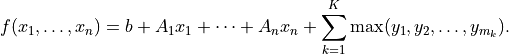
$f(x_1,\ldots,x_n) = b + A_1 x_1 + \cdots + A_n x_n + \sum_{k=1}^K \max (y_1, y_2, \ldots, y_{m_k}).$

The maximum in this expression is a componentwise maximum of its vector arguments, which can be constant vectors, variables, affine functions or convex piecewise-linear functions. The general expression for a concave piecewise-linear function is

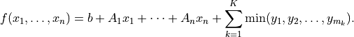
$f(x_1,\ldots,x_n) = b + A_1 x_1 + \cdots + A_n x_n + \sum_{k=1}^K \min (y_1, y_2, \ldots, y_{m_k}).$

Here the arguments of the min can be constants, variables, affine functions or concave piecewise-linear functions.

Piecewise-linear functions can be created using the following operations.

Maximum

If the arguments in f = max(y1, y2, ...) do not include any variables or functions, then the Python built-in max is evaluated.

If one or more of the arguments are variables or functions, max returns a piecewise-linear function defined as the elementwise maximum of its arguments. In other words, f[k] = max(y1[k], y2[k], ...) for k = 0, …, len(f) - 1. The length of f is equal to the maximum of the lengths of the arguments. Each argument must have length equal to len(f) or length one. Arguments with length one are interpreted as vectors of length len(f) with identical entries.

The arguments can be scalars of type integer or float, dense 'd' matrices with one column, variables, affine functions or convex piecewise-linear functions.

With one argument, f = max(u) is interpreted as f = max(u[0], u[1], ..., u[len(u)-1]).

Minimum

Similar to max but returns a concave piecewise-linear function. The arguments can be scalars of type integer or float, dense 'd' matrices with one column, variables, affine functions or concave piecewise-linear functions.

Absolute value

If u is a variable or affine function then f = abs(u) returns the convex piecewise-linear function max(u, -u).

Unary plus and minus

+f creates a copy of f. -f is a concave piecewise-linear function if f is convex and a convex piecewise-linear function if f is concave.

Addition and subtraction

Sums and differences involving piecewise-linear functions are allowed if they result in convex or concave functions. For example, one can add two convex or two concave functions, but not a convex and a concave function. The command sum(f) is equivalent to f[0] + f[1] + ... + f[len(f) - 1].

Multiplication

Scalar multiplication a * f of a piecewise-linear function f is defined if a is an integer, float, 1 by 1 'd' matrix. Matrix-matrix multiplications a * f or f * a are only defined if a is a dense or sparse 1 by 1 matrix.

Indexing and slicing

Piecewise-linear functions admit single-argument indexing of the four types described in the section Indexing and Slicing. The result of an indexing or slicing operation is a new piecewise-linear function.

In the following example, f is the 1-norm of a vector variable x of length 10, g is its infinity-norm, and h is the function

$h(x) = \sum_k \phi(x[k]), \qquad \phi(u) = \left\{\begin{array}{ll} 0 & |u| \leq 1 \\ |u|-1 & 1 \leq |u| \leq 2 \\ 2|u|-3 & |u| \geq 2. \end{array}\right.$

>>> from cvxopt.modeling import variable, max
>>> x = variable(10, 'x')
>>> f = sum(abs(x))
>>> g = max(abs(x))
>>> h = sum(max(0, abs(x)-1, 2*abs(x)-3))

In-place operations: If f is piecewise-linear then the in-place operations f += u, f -= u, f *= u, f /= u are defined if the corresponding expanded operations f = f + u, f = f - u, f = f * u, and f = f/u are defined and if they do not change the length of f.

Constraints

Linear equality and inequality constraints of the form

$f(x_1,\ldots,x_n) = 0, \qquad f(x_1,\ldots,x_n) \preceq 0,$

where $f$ is a convex function, are represented by constraint objects. Equality constraints are created by expressions of the form

f1 == f2

Here f1 and f2 can be any objects for which the difference f1 - f2 yields an affine function. Inequality constraints are created by expressions of the form

f1 <= f2
f2 >= f1

where f1 and f2 can be any objects for which the difference f1 - f2 yields a convex piecewise-linear function. The comparison operators first convert the expressions to f1 - f2 == 0, resp., f1 - f2 <= 0, and then return a new constraint object with constraint function f1 - f2.

In the following example we create three constraints

$\newcommand{\ones}{{\bf 1}} 0 \preceq x \preceq \ones, \qquad \ones^T x = 2,$

for a variable of length 5.

>>> x = variable(5,'x')
>>> c1 = (x <= 1)
>>> c2 = (x >= 0)
>>> c3 = (sum(x) == 2)

The built-in function len returns the dimension of the constraint function.

Constraints have four public attributes.

constraint.type: Returns '=' if the constraint is an equality constraint, and ‘<’ if the constraint is an inequality constraint.

constraint.value: Returns the value of the constraint function.

constraint.multiplier: For a constraint c, c.multiplier is a variable object of dimension len(c). It is used to represent the Lagrange multiplier or dual variable associated with the constraint. Its value is initialized as None, and can be modified by making an assignment to c.multiplier.value.

constraint.name: The name of the constraint. Changing the name of a constraint also changes the name of the multiplier of c. For example, the command c.name = 'newname' also changes c.multiplier.name to 'newname_mul'.

Optimization Problems

Optimization problems are be constructed by calling the following function.

cvxopt.modeling.op([objective[, constraints[, name]]])

The first argument specifies the objective function to be minimized. It can be an affine or convex piecewise-linear function with length 1, a variable with length 1, or a scalar constant (integer, float, or 1 by 1 dense 'd' matrix). The default value is 0.0.

The second argument is a single constraint, or a list of constraint objects. The default value is an empty list.

The third argument is a string with a name for the problem. The default value is the empty string.

The following attributes and methods are useful for examining and modifying optimization problems.

op.objective: The objective or cost function. One can write to this attribute to change the objective of an existing problem.

op.variables(): Returns a list of the variables of the problem.

op.constraints(): Returns a list of the constraints.

op.inequalities(): Returns a list of the inequality constraints.

op.equalities(): Returns a list of the equality constraints.

op.delconstraint(c): Deletes constraint c from the problem.

op.addconstraint(c): Adds constraint c to the problem.

An optimization problem with convex piecewise-linear objective and constraints can be solved by calling the method solve.

op.solve([format[, solver]])

This function converts the optimization problem to a linear program in matrix form and then solves it using the solver described in the section Linear Programming.

The first argument is either 'dense' or 'sparse', and denotes the matrix types used in the matrix representation of the LP. The default value is 'dense'.

The second argument is either None, 'glpk', or 'mosek', and selects one of three available LP solvers: the default solver written in Python, the GLPK solver (if installed) or the MOSEK LP solver (if installed); see the section Linear Programming. The default value is None.

The solver reports the outcome of optimization by setting the attribute self.status and by modifying the value attributes of the variables and the constraint multipliers of the problem.

If the problem is solved to optimality, self.status is set to 'optimal'. The value attributes of the variables in the problem are set to their computed solutions, and the value attributes of the multipliers of the constraints of the problem are set to the computed dual optimal solution.
If it is determined that the problem is infeasible, self.status is set to 'primal infeasible'. The value attributes of the variables are set to None. The value attributes of the multipliers of the constraints of the problem are set to a certificate of primal infeasibility. With the 'glpk' option, solve does not provide certificates of infeasibility.
If it is determined that the problem is dual infeasible, self.status is set to 'dual infeasible'. The value attributes of the multipliers of the constraints of the problem are set to None. The value attributes of the variables are set to a certificate of dual infeasibility. With the 'glpk' option, solve does not provide certificates of infeasibility.
If the problem was not solved successfully, self.status is set to 'unknown'. The value attributes of the variables and the constraint multipliers are set to None.

We refer to the section Linear Programming for details on the algorithms and the different solver options.

As an example we solve the LP

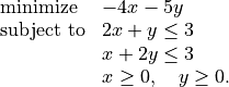
$\begin{array}{ll} \mbox{minimize} & -4x - 5y \\ \mbox{subject to} & 2x +y \leq 3 \\ & x +2y \leq 3 \\ & x \geq 0, \quad y \geq 0. \end{array}$

>>> from cvxopt.modeling import op
>>> x = variable()
>>> y = variable()
>>> c1 = ( 2*x+y <= 3 )
>>> c2 = ( x+2*y <= 3 )
>>> c3 = ( x >= 0 )
>>> c4 = ( y >= 0 )
>>> lp1 = op(-4*x-5*y, [c1,c2,c3,c4])
>>> lp1.solve()
>>> lp1.status
'optimal'
>>> print(lp1.objective.value())
[-9.00e+00]
>>> print(x.value)
[ 1.00e+00]
>>> print(y.value)
[ 1.00e+00]
>>> print(c1.multiplier.value)
[ 1.00e+00]
>>> print(c2.multiplier.value)
[ 2.00e+00]
>>> print(c3.multiplier.value)
[ 2.87e-08]
>>> print(c4.multiplier.value)
[ 2.80e-08]

We can solve the same LP in matrix form as follows.

>>> from cvxopt.modeling import op, dot
>>> x = variable(2)
>>> A = matrix([[2.,1.,-1.,0.], [1.,2.,0.,-1.]])
>>> b = matrix([3.,3.,0.,0.])
>>> c = matrix([-4.,-5.])
>>> ineq = ( A*x <= b )
>>> lp2 = op(dot(c,x), ineq)
>>> lp2.solve()
>>> print(lp2.objective.value())
[-9.00e+00]
>>> print(x.value)
[ 1.00e+00]
[ 1.00e+00]
>>> print(ineq.multiplier.value)
[1.00e+00]
[2.00e+00]
[2.87e-08]
[2.80e-08]

The op class also includes two methods for writing and reading files in MPS format.

tofile(filename) :noindex:: If the problem is an LP, writes it to the file filename using the MPS format. Row and column labels are assigned based on the variable and constraint names in the LP.

fromfile(filename) :noindex:: Reads the LP from the file filename. The file must be a fixed-format MPS file. Some features of the MPS format are not supported: comments beginning with dollar signs, the row types ‘DE’, ‘DL’, ‘DG’, and ‘DN’, and the capability of reading multiple righthand side, bound or range vectors.

Examples

Norm and Penalty Approximation

In the first example we solve the norm approximation problems

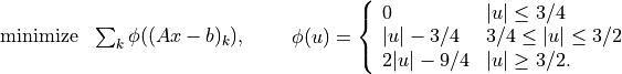
$\begin{array}{ll} \mbox{minimize} & \|Ax - b\|_\infty, \end{array} \qquad \begin{array}{ll} \mbox{minimize} & \|Ax - b\|_1 \end{array},$

and the penalty approximation problem

$\begin{array}{ll} \mbox{minimize} & \sum_k \phi((Ax-b)_k), \end{array} \qquad \phi(u) = \left\{\begin{array}{ll} 0 & |u| \leq 3/4 \\ |u|-3/4 & 3/4 \leq |u| \leq 3/2 \\ 2|u|-9/4 & |u| \geq 3/2. \end{array}\right.$

We use randomly generated data.

The code uses the Matplotlib package for plotting the histograms of the residual vectors for the two solutions. It generates the figure shown below.

from cvxopt import normal
from cvxopt.modeling import variable, op, max, sum
import pylab

m, n = 500, 100
A = normal(m,n)
b = normal(m)

x1 = variable(n)
op(max(abs(A*x1-b))).solve()

x2 = variable(n)
op(sum(abs(A*x2-b))).solve()

x3 = variable(n)
op(sum(max(0, abs(A*x3-b)-0.75, 2*abs(A*x3-b)-2.25))).solve()

pylab.subplot(311)
pylab.hist(A*x1.value-b, m/5)
pylab.subplot(312)
pylab.hist(A*x2.value-b, m/5)
pylab.subplot(313)
pylab.hist(A*x3.value-b, m/5)
pylab.show()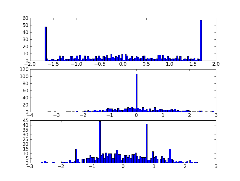

Equivalently, we can formulate and solve the problems as LPs.

t = variable()
x1 = variable(n)
op(t, [-t <= A*x1-b, A*x1-b<=t]).solve()

u = variable(m)
x2 = variable(n)
op(sum(u), [-u <= A*x2+b, A*x2+b <= u]).solve()

v = variable(m)
x3 = variable(n)
op(sum(v), [v >= 0, v >= A*x3+b-0.75, v >= -(A*x3+b)-0.75, v >= 2*(A*x3-b)-2.25, v >= -2*(A*x3-b)-2.25]).solve()

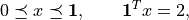
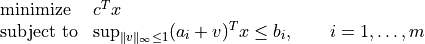
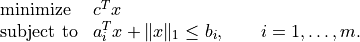
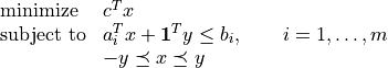
Robust Linear Programming

The robust LP

$\begin{array}{ll} \mbox{minimize} & c^T x \\ \mbox{subject to} & \sup_{\|v\|_\infty \leq 1} (a_i+v)^T x \leq b_i, \qquad i=1,\ldots,m \end{array}$

is equivalent to the problem

$\begin{array}{ll} \mbox{minimize} & c^Tx \\ \mbox{subject to} & a_i^Tx + \|x\|_1 \leq b_i, \qquad i=1,\ldots,m. \end{array}$

The following code computes the solution and the solution of the equivalent LP

$\newcommand{\ones}{{\bf 1}} \begin{array}{ll} \mbox{minimize} & c^Tx \\ \mbox{subject to} & a_i^Tx + \ones^Ty \leq b_i, \qquad i=1,\ldots,m \\ & -y \preceq x \preceq y \end{array}$

for randomly generated data.

from cvxopt import normal, uniform
from cvxopt.modeling import variable, dot, op, sum

m, n = 500, 100
A = normal(m,n)
b = uniform(m)
c = normal(n)

x = variable(n)
op(dot(c,x), A*x+sum(abs(x)) <= b).solve()

x2 = variable(n)
y = variable(n)
op(dot(c,x2), [A*x2+sum(y) <= b, -y <= x2, x2 <= y]).solve()

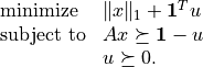
1-Norm Support Vector Classifier

The following problem arises in classification:

$\newcommand{\ones}{{\bf 1}} \begin{array}{ll} \mbox{minimize} & \|x\|_1 + \ones^Tu \\ \mbox{subject to} & Ax \succeq \ones -u \\ & u \succeq 0. \end{array}$

It can be solved as follows.
x = variable(A.size[1],'x')
u = variable(A.size[0],'u')
op(sum(abs(x)) + sum(u), [A*x >= 1-u, u >= 0]).solve()
An equivalent unconstrained formulation is
x = variable(A.size[1],'x')
op(sum(abs(x)) + sum(max(0,1-A*x))).solve()