Sparse Linear Equations

In this section we describe routines for solving sparse sets of linear equations.

A real symmetric or complex Hermitian sparse matrix is stored as an spmatrix object X of size ( $n$ , $n$ ) and an additional character argument uplo with possible values 'L' and 'U'. If uplo is 'L', the lower triangular part of X contains the lower triangular part of the symmetric or Hermitian matrix, and the upper triangular matrix of X is ignored. If uplo is 'U', the upper triangular part of X contains the upper triangular part of the matrix, and the lower triangular matrix of X is ignored.

A general sparse square matrix of order $n$ is represented by an spmatrix object of size ( $n$ , $n$ ).

Dense matrices, which appear as right-hand sides of equations, are stored using the same conventions as in the BLAS and LAPACK modules.

Matrix Orderings

CVXOPT includes an interface to the AMD library for computing approximate minimum degree orderings of sparse matrices.

General Linear Equations

The module cvxopt.umfpack includes four functions for solving sparse non-symmetric sets of linear equations. They call routines from the UMFPACK library, with all control options set to the default values described in the UMFPACK user guide.

See also

T. A. Davis, Algorithm 832: UMFPACK – an unsymmetric-pattern multifrontal method with a column pre-ordering strategy, ACM Transactions on Mathematical Software, 30(2), 196-199, 2004.

cvxopt.umfpack.linsolve(A, B[, trans = 'N'])

Solves a sparse set of linear equations

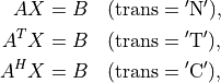
$AX & = B \quad (\mathrm{trans} = \mathrm{'N'}), \\ A^TX & = B \quad (\mathrm{trans} = \mathrm{'T'}), \\ A^HX & = B \quad (\mathrm{trans} = \mathrm{'C'}),$

where $A$ is a sparse matrix and $B$ is a dense matrix. The arguments A and B must have the same type ('d' or 'z') as A. On exit B contains the solution. Raises an ArithmeticError if the coefficient matrix is singular.

In the following example we solve an equation with coefficient matrix

(1) $A = \left[\begin{array}{rrrrr} 2 & 3 & 0 & 0 & 0 \\ 3 & 0 & 4 & 0 & 6 \\ 0 &-1 &-3 & 2 & 0 \\ 0 & 0 & 1 & 0 & 0 \\ 0 & 4 & 2 & 0 & 1 \end{array}\right].$

>>> from cvxopt import spmatrix, matrix, umfpack
>>> V = [2, 3, 3, -1, 4, 4, -3, 1, 2, 2, 6, 1]
>>> I = [0, 1, 0,  2, 4, 1,  2, 3, 4, 2, 1, 4]
>>> J = [0, 0, 1,  1, 1, 2,  2, 2, 2, 3, 4, 4]
>>> A = spmatrix(V,I,J)
>>> B = matrix(1.0, (5,1))
>>> umfpack.linsolve(A,B)
>>> print(B)
[ 5.79e-01]
[-5.26e-02]
[ 1.00e+00]
[ 1.97e+00]
[-7.89e-01]

The function linsolve is equivalent to the following three functions called in sequence.

cvxopt.umfpack.symbolic(A): Reorders the columns of A to reduce fill-in and performs a symbolic LU factorization. A is a sparse, possibly rectangular, matrix. Returns the symbolic factorization as an opaque C object that can be passed on to numeric.

cvxopt.umfpack.numeric(A, F): Performs a numeric LU factorization of a sparse, possibly rectangular, matrix A. The argument F is the symbolic factorization computed by symbolic applied to the matrix A, or another sparse matrix with the same sparsity pattern, dimensions, and type. The numeric factorization is returned as an opaque C object that that can be passed on to solve. Raises an ArithmeticError if the matrix is singular.

cvxopt.umfpack.solve(A, F, B[, trans = 'N'])

Solves a set of linear equations

$AX & = B \quad (\mathrm{trans} = \mathrm{'N'}), \\ A^TX & = B \quad (\mathrm{trans} = \mathrm{'T'}), \\ A^HX & = B \quad (\mathrm{trans} = \mathrm{'C'}),$

where $A$ is a sparse matrix and $B$ is a dense matrix. The arguments A and B must have the same type. The argument F is a numeric factorization computed by numeric. On exit B is overwritten by the solution.

These separate functions are useful for solving several sets of linear equations with the same coefficient matrix and different right-hand sides, or with coefficient matrices that share the same sparsity pattern. The symbolic factorization depends only on the sparsity pattern of the matrix, and not on the numerical values of the nonzero coefficients. The numerical factorization on the other hand depends on the sparsity pattern of the matrix and on its the numerical values.

As an example, suppose $A$ is the matrix (1) and

$B = \left[\begin{array}{rrrrr} 4 & 3 & 0 & 0 & 0 \\ 3 & 0 & 4 & 0 & 6 \\ 0 &-1 &-3 & 2 & 0 \\ 0 & 0 & 1 & 0 & 0 \\ 0 & 4 & 2 & 0 & 2 \end{array}\right],$

which differs from $A$ in its first and last entries. The following code computes

$\newcommand{\ones}{\mathbf 1} x = A^{-T}B^{-1}A^{-1}\ones.$

>>> from cvxopt import spmatrix, matrix, umfpack
>>> VA = [2, 3, 3, -1, 4, 4, -3, 1, 2, 2, 6, 1]
>>> VB = [4, 3, 3, -1, 4, 4, -3, 1, 2, 2, 6, 2]
>>> I =  [0, 1, 0,  2, 4, 1,  2, 3, 4, 2, 1, 4]
>>> J =  [0, 0, 1,  1, 1, 2,  2, 2, 2, 3, 4, 4]
>>> A = spmatrix(VA, I, J)
>>> B = spmatrix(VB, I, J)
>>> x = matrix(1.0, (5,1))
>>> Fs = umfpack.symbolic(A)
>>> FA = umfpack.numeric(A, Fs)
>>> FB = umfpack.numeric(B, Fs)
>>> umfpack.solve(A, FA, x)
>>> umfpack.solve(B, FB, x)
>>> umfpack.solve(A, FA, x, trans='T')
>>> print(x)
[ 5.81e-01]
[-2.37e-01]
[ 1.63e+00]
[ 8.07e+00]
[-1.31e-01]

Positive Definite Linear Equations

cvxopt.cholmod is an interface to the Cholesky factorization routines of the CHOLMOD package. It includes functions for Cholesky factorization of sparse positive definite matrices, and for solving sparse sets of linear equations with positive definite matrices. The routines can also be used for computing LDL^T (or LDL^H factorizations of symmetric indefinite matrices (with $L$ unit lower-triangular and $D$ diagonal and nonsingular) if such a factorization exists.

See also

Y. Chen, T. A. Davis, W. W. Hager, S. Rajamanickam, Algorithm 887: CHOLMOD, Supernodal Sparse Cholesky Factorization and Update/Downdate, ACM Transactions on Mathematical Software, 35(3), 22:1-22:14, 2008.

cvxopt.cholmod.linsolve(A, B[, p = None, uplo = 'L'])

Solves

$AX = B$

with $A$ sparse and real symmetric or complex Hermitian.

B is a dense matrix of the same type as A. On exit it is overwritten with the solution. The argument p is an integer matrix with length equal to the order of $A$ , and specifies an optional reordering. See the comment on options['nmethods'] for details on which ordering is used by CHOLMOD.

Raises an ArithmeticError if the factorization does not exist.

As an example, we solve

(2) $\left[ \begin{array}{rrrr} 10 & 0 & 3 & 0 \\ 0 & 5 & 0 & -2 \\ 3 & 0 & 5 & 0 \\ 0 & -2 & 0 & 2 \end{array}\right] X = \left[ \begin{array}{cc} 0 & 4 \\ 1 & 5 \\ 2 & 6 \\ 3 & 7 \end{array} \right].$

>>> from cvxopt import matrix, spmatrix, cholmod
>>> A = spmatrix([10, 3, 5, -2, 5, 2], [0, 2, 1, 3, 2, 3], [0, 0, 1, 1, 2, 3])
>>> X = matrix(range(8), (4,2), 'd')
>>> cholmod.linsolve(A,X)
>>> print(X)
[-1.46e-01  4.88e-02]
[ 1.33e+00  4.00e+00]
[ 4.88e-01  1.17e+00]
[ 2.83e+00  7.50e+00]

cvxopt.cholmod.splinsolve(A, B[, p = None, uplo = 'L']): Similar to linsolve except that B is an spmatrix and that the solution is returned as an output argument (as a new spmatrix). B is not modified. See the comment on options['nmethods'] for details on which ordering is used by CHOLMOD.

The following code computes the inverse of the coefficient matrix in (2) as a sparse matrix.

>>> X = cholmod.splinsolve(A, spmatrix(1.0,range(4),range(4)))
>>> print(X)
[ 1.22e-01     0     -7.32e-02     0    ]
[    0      3.33e-01     0      3.33e-01]
[-7.32e-02     0      2.44e-01     0    ]
[    0      3.33e-01     0      8.33e-01]

The functions linsolve and splinsolve are equivalent to symbolic and numeric called in sequence, followed by solve, respectively, spsolve.

cvxopt.cholmod.symbolic(A[, p = None, uplo = 'L'])

Performs a symbolic analysis of a sparse real symmetric or complex Hermitian matrix $A$ for one of the two factorizations:

(3) $PAP^T = LL^T, \qquad PAP^T = LL^H,$

and

(4) $PAP^T = LDL^T, \qquad PAP^T = LDL^H,$

where $P$ is a permutation matrix, $L$ is lower triangular (unit lower triangular in the second factorization), and $D$ is nonsingular diagonal. The type of factorization depends on the value of options['supernodal'] (see below).

If uplo is 'L', only the lower triangular part of A is accessed and the upper triangular part is ignored. If uplo is 'U', only the upper triangular part of A is accessed and the lower triangular part is ignored.

The symbolic factorization is returned as an opaque C object that can be passed to numeric.

See the comment on options['nmethods'] for details on which ordering is used by CHOLMOD.

cvxopt.cholmod.numeric(A, F)

Performs a numeric factorization of a sparse symmetric matrix as (3) or (4). The argument F is the symbolic factorization computed by symbolic applied to the matrix A, or to another sparse matrix with the same sparsity pattern and typecode, or by numeric applied to a matrix with the same sparsity pattern and typecode as A.

If F was created by a symbolic with uplo equal to 'L', then only the lower triangular part of A is accessed and the upper triangular part is ignored. If it was created with uplo equal to 'U', then only the upper triangular part of A is accessed and the lower triangular part is ignored.

On successful exit, the factorization is stored in F. Raises an ArithmeticError if the factorization does not exist.

cvxopt.cholmod.solve(F, B[, sys = 0])

Solves one of the following linear equations where B is a dense matrix and F is the numeric factorization (3) or (4) computed by numeric. sys is an integer with values between 0 and 8.

`sys`	equation
0	$AX = B$
1	$LDL^TX = B$
2	$LDX = B$
3	$DL^TX=B$
4	$LX=B$
5	$L^TX=B$
6	$DX=B$
7	$P^TX=B$
8	$PX=B$

(If F is a Cholesky factorization of the form (3), $D$ is an identity matrix in this table. If A is complex, $L^T$ should be replaced by $L^H$ .)

The matrix B is a dense 'd' or 'z' matrix, with the same type as A. On exit it is overwritten by the solution.

cvxopt.cholmod.spsolve(F, B[, sys = 0]): Similar to solve, except that B is a class:spmatrix, and the solution is returned as an output argument (as an spmatrix). B must have the same typecode as A.

For the same example as above:

>>> X = matrix(range(8), (4,2), 'd')
>>> F = cholmod.symbolic(A)
>>> cholmod.numeric(A, F)
>>> cholmod.solve(F, X)
>>> print(X)
[-1.46e-01  4.88e-02]
[ 1.33e+00  4.00e+00]
[ 4.88e-01  1.17e+00]
[ 2.83e+00  7.50e+00]

cvxopt.cholmod.diag(F): Returns the diagonal elements of the Cholesky factor $L$ in (3), as a dense matrix of the same type as A. Note that this only applies to Cholesky factorizations. The matrix $D$ in an LDL^T factorization can be retrieved via solve with sys equal to 6.

In the functions listed above, the default values of the control parameters described in the CHOLMOD user guide are used, except for Common.print which is set to 0 instead of 3 and Common.supernodal which is set to 2 instead of 1. These parameters (and a few others) can be modified by making an entry in the dictionary cholmod.options. The meaning of the options options['supernodal'] and options['nmethods'] is summarized as follows (and described in detail in the CHOLMOD user guide).

options['supernodal']: If equal to 0, a factorization (4) is computed using a simplicial algorithm. If equal to 2, a factorization (3) is computed using a supernodal algorithm. If equal to 1, the most efficient of the two factorizations is selected, based on the sparsity pattern. Default: 2.
options['nmethods']: The default ordering used by the CHOLMOD is the ordering in the AMD library, but depending on the value of options['nmethods']. other orderings are also considered. If nmethods is equal to 2, the ordering specified by the user and the AMD ordering are compared, and the best of the two orderings is used. If the user does not specify an ordering, the AMD ordering is used. If equal to 1, the user must specify an ordering, and the ordering provided by the user is used. If equal to 0, all available orderings are compared and the best ordering is used. The available orderings include the AMD ordering, the ordering specified by the user (if any), and possibly other orderings if they are installed during the CHOLMOD installation. Default: 0.

As an example that illustrates diag and the use of cholmod.options, we compute the logarithm of the determinant of the coefficient matrix in (2) by two methods.

>>> import math
>>> from cvxopt.cholmod import options
>>> from cvxopt import log
>>> F = cholmod.symbolic(A)
>>> cholmod.numeric(A, F)
>>> print(2.0 * sum(log(cholmod.diag(F))))
5.50533153593
>>> options['supernodal'] = 0
>>> F = cholmod.symbolic(A)
>>> cholmod.numeric(A, F)
>>> Di = matrix(1.0, (4,1))
>>> cholmod.solve(F, Di, sys=6)
>>> print(-sum(log(Di)))
5.50533153593

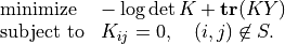
Example: Covariance Selection

This example illustrates the use of the routines for sparse Cholesky factorization. We consider the problem

(5) $\newcommand{\Tr}{\mathop{\bf tr}} \begin{array}{ll} \mbox{minimize} & -\log\det K + \Tr(KY) \\ \mbox{subject to} & K_{ij}=0,\quad (i,j) \not \in S. \end{array}$

The optimization variable is a symmetric matrix $K$ of order $n$ and the domain of the problem is the set of positive definite matrices. The matrix $Y$ and the index set $S$ are given. We assume that all the diagonal positions are included in $S$ . This problem arises in maximum likelihood estimation of the covariance matrix of a zero-mean normal distribution, with constraints that specify that pairs of variables are conditionally independent.

We can express $K$ as

$\newcommand{\diag}{\mathop{\bf diag}} K(x) = E_1\diag(x)E_2^T+E_2\diag(x)E_1^T$

where $x$ are the nonzero elements in the lower triangular part of $K$ , with the diagonal elements scaled by 1/2, and

$E_1 = \left[ \begin{array}{cccc} e_{i_1} & e_{i_2} & \cdots & e_{i_q} \end{array}\right], \qquad E_2 = \left[ \begin{array}{cccc} e_{j_1} & e_{j_2} & \cdots & e_{j_q} \end{array}\right],$

where ( $i_k$ , $j_k$ ) are the positions of the nonzero entries in the lower-triangular part of $K$ . With this notation, we can solve problem (5) by solving the unconstrained problem

$\newcommand{\Tr}{\mathop{\bf tr}} \begin{array}{ll} \mbox{minimize} & f(x) = -\log\det K(x) + \Tr(K(x)Y). \end{array}$

The code below implements Newton’s method with a backtracking line search. The gradient and Hessian of the objective function are given by

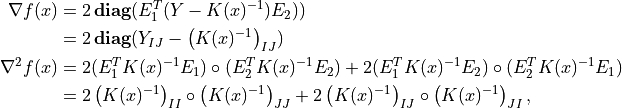
$\newcommand{\diag}{\mathop{\bf diag}} \begin{split} \nabla f(x) & = 2 \diag( E_1^T (Y - K(x)^{-1}) E_2)) \\ & = 2\diag(Y_{IJ} - \left(K(x)^{-1}\right)_{IJ}) \\ \nabla^2 f(x) & = 2 (E_1^T K(x)^{-1} E_1) \circ (E_2^T K(x)^{-1} E_2) + 2 (E_1^T K(x)^{-1} E_2) \circ (E_2^T K(x)^{-1} E_1) \\ & = 2 \left(K(x)^{-1}\right)_{II} \circ \left(K(x)^{-1}\right)_{JJ} + 2 \left(K(x)^{-1}\right)_{IJ} \circ \left(K(x)^{-1}\right)_{JI}, \end{split}$

where $\circ$ denotes Hadamard product.

from cvxopt import matrix, spmatrix, log, mul, blas, lapack, amd, cholmod

def covsel(Y):
    """
    Returns the solution of

         minimize    -log det K + Tr(KY)
         subject to  K_{ij}=0,  (i,j) not in indices listed in I,J.

    Y is a symmetric sparse matrix with nonzero diagonal elements.
    I = Y.I,  J = Y.J.
    """

    I, J = Y.I, Y.J
    n, m = Y.size[0], len(I)
    N = I + J*n         # non-zero positions for one-argument indexing
    D = [k for k in range(m) if I[k]==J[k]]  # position of diagonal elements

    # starting point: symmetric identity with nonzero pattern I,J
    K = spmatrix(0.0, I, J)
    K[::n+1] = 1.0

    # Kn is used in the line search
    Kn = spmatrix(0.0, I, J)

    # symbolic factorization of K
    F = cholmod.symbolic(K)

    # Kinv will be the inverse of K
    Kinv = matrix(0.0, (n,n))

    for iters in range(100):

        # numeric factorization of K
        cholmod.numeric(K, F)
        d = cholmod.diag(F)

        # compute Kinv by solving K*X = I
        Kinv[:] = 0.0
        Kinv[::n+1] = 1.0
        cholmod.solve(F, Kinv)

        # solve Newton system
        grad = 2*(Y.V - Kinv[N])
        hess = 2*(mul(Kinv[I,J],Kinv[J,I]) + mul(Kinv[I,I],Kinv[J,J]))
        v = -grad
        lapack.posv(hess,v)

        # stopping criterion
        sqntdecr = -blas.dot(grad,v)
        print("Newton decrement squared:%- 7.5e" %sqntdecr)
        if (sqntdecr < 1e-12):
            print("number of iterations: ", iters+1)
            break

        # line search
        dx = +v
        dx[D] *= 2      # scale the diagonal elems
        f = -2.0 * sum(log(d))    # f = -log det K
        s = 1
        for lsiter in range(50):
            Kn.V = K.V + s*dx
            try:
                cholmod.numeric(Kn, F)
            except ArithmeticError:
                s *= 0.5
            else:
                d = cholmod.diag(F)
                fn = -2.0 * sum(log(d)) + 2*s*blas.dot(v,Y.V)
                if (fn < f - 0.01*s*sqntdecr):
                     break
                s *= 0.5

        K.V = Kn.V

    return K